

A sentence to be used as news excerpt. This should be short enough to fit nicely the carousel on the home page.
R Markdown
Refer to the R Studio website for a comprehensive introduction to R Markdown.
Also refer to the conventional markdown news post template for general instructions and guidelines about writing news posts, such as details about including non-R-generated pictures, links, etc.
Code chunks
This is an example of R chunk labeled my-first-chunk (it is recommended to provide a label for all chunks), without any special option.
# some code
(a <- 10)
## [1] 10
b <- sqrt(a)
a + b
## [1] 13.16228
You can fine-tune the behavior/results using chunk options, e.g. echo=FALSE, eval=FALSE, include=FALSE, results='hide', error=TRUE.
Get used to write consistently-formatted, tidy R code, especially concerning spacing and parentheses (see e.g. the ‘Syntax’ section in Hadley’s style guide).
The following is an example of un-tidy, poorly formatted code:
fun <-function(x  =NULL)
{
  if(length(x)!=0)  {
    x<-0.0;
  }
  return( x )
}
fun  (0.0)
## [1] 0
Besides writing tidy code yourself, you might want to use the tidy chunk option, causing the R code to be re-formatted in a tidy way. (This can be enabled for all code chunks in the initial setup chunk. Note that the tidy chunk option requires the package formatR, otherwise the code will remain as is and you will just get a warning when knitting.)
fun <- function(x = NULL) {
  if (length(x) != 0) {
    x <- 0
  }
  return(x)
}
fun(0)
Note that previous chunks can be re-called by label later in the document, as in the tidy chunk above.
You should avoid exceeding 80 characters per line, since the font size for code chunks is tuned to fit 80 characters without horizontal scrolling:
x <- "
12345678901234567890123456789012345678901234567890123456789012345678901234567890
"
Copy button
As showcased in the plain Markdown post template, code blocks include a “Copy to Clipboard” button by default. For an R Markdown code chunk, {: .no-code-copy } can still be added below the chunk.
hello_world <- "Hello World!"
print(hello_world)
## [1] "Hello World!"
Note that, for code chunks producing output and having the option collapse=FALSE (possibly set via knitr::opts_chunk$set()), two code blocks are produced: one for the source code and one for the output. Using {: .no-code-copy } would only disable the copy button for the output, which is usually desired.
hello_world <- "Hello World!"
print(hello_world)
## [1] "Hello World!"
If you need to disable the copy button for the source code, two dedicated R Markdown code chunks can be used: one with results='hide' for the source code, and an empty one using the same label and echo=FALSE for the output.
hello_world <- "Hello World!"
print(hello_world)
## [1] "Hello World!"
Supporting (source) files
If the R Markdown post needs some supporting files, to be used within code chunks or as code chunks (e.g. R scripts), place them in the same post-specific directory so they can be accessed via relative paths. In particular, it is possible to define stand-alone scripts, e.g. myFun.R, and use knitr::read_chunk(<FILE>, labels = <LABEL>) in a first non-included chunk, before re-calling the content by label in a second chunk.
## myFun.R
#' @title My function.
#' @description My function.
#' @param arg1 My first argument.
#' @param arg2 My second argument.
#' @return My return value.
#' @export
myFun <- function(arg1, arg2) {
  "My return value"
}
Figures
Figures generated by plotting in any R code chunk are automatically generated and linked (note echo=FALSE to show only the image and not the underlying code). We usually want to specify an explicit figure caption via fig.cap='...' to override the default “plot of chunk <chunk-label>”
The classes described for conventional Markdown pictures, can and should be specified (possibly alongside CSS styling) as chunk option
out.extra='class="img-responsive ..." style="..."'. Note that generated figures are already centered by default.
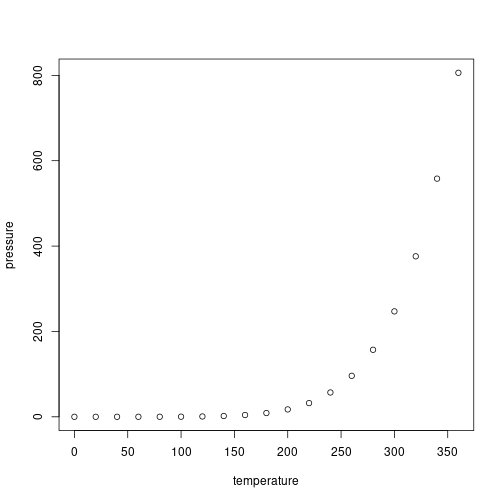
Example plot
Size tuning
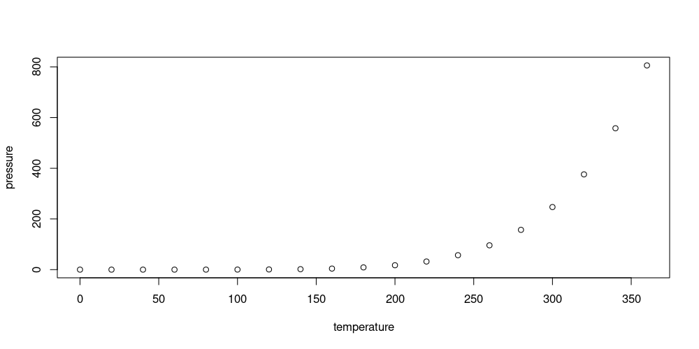
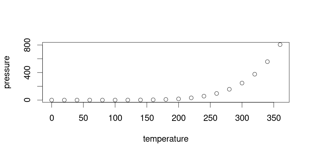
The pixel size of the generated image is best controlled using the fig.width, fig.asp, dpi chunk options. Note that dpi affects the relative size of elements like text, lines, points, margins: this can be tuned via dev.args=list(pointsize = <N>) (or similarly in the plotting code). For instance, both pictures below are generated with fig.width=10, fig.asp=0.5, dpi=100, resulting in 1000x500 pixels, and displayed with out.extra='class="img-responsive img-large"'. The second picture is however generated with dev.args=list(pointsize = 50).
Example plot
Example plot
Interactive widgets
R code chunks producing interactive widgets, such as leaflet maps or plots generated with plotly, typically relies on JavaScript and cannot be included as-is in the rendered post. Instead, a static screenshot is included using PhantomJS, which must be available and can be installed via webshot::install_phantomjs().
The size and geometry of the static snapshot image is still controlled by chunk options as described above. Note however that, in many cases, dpi would only control the image pixel size (as dpi*fig.width), with the size of the elements controlled by the widget-generating code (dev.args not having any effect). Below is an example 1000x500 snapshot of a plotly graph with fig.width=10, fig.asp=0.5, dpi=100, and plotly-specific element size tuning.
plotly::plot_ly(
  pressure, x = ~temperature, y = ~pressure,
  type = 'scatter', mode = 'lines+markers',
  marker = list(size = 15), line = list(width = 6)
) %>% plotly::layout(
  font = list(size = 30),
  xaxis = list(zerolinewidth = 4),
  yaxis = list(zerolinewidth = 4)
)

Parameters
Parameters declared in the params field within the YAML header are accessible as read-only list called params.
The list can be used inline (DUMMY) or in R code chunks:
params$dummy
## [1] "DUMMY"